1 - Fundamentals of microalgae-based processes.

1.4 - Key concepts in photobioreactor (PBR) design

This course focuses on the design and operation of industrial microalgae cultures carried out in Photobioreactors (PBRs). The objective of this type of culture is very different from that of laboratory cultures, as it is oriented towards:

• Producing the maximum amount of biomass per unit of culture volume (PBR volume).

• Consuming the minimum resources (medium, gases such as CO2, pumping/agitation energy, gas sparging, etc.).

• Maintaining the culture over the long term: stability.

• Maximising the content of products of interest.

To achieve this, we will handle the following concepts quantitatively, which is what distinguishes mass cultures from laboratory cultures.

- Specific growth rate

The specific growth rate $(\mu)$ is the parameter that most faithfully represents a microorganism's capacity to produce biomass. As already discussed in Section 1.1, its definition is:

$$\begin{align} \large \mu= \frac{1}{C_b} \cdot \frac{dC_b}{dt} \tag{1.4.1} \end{align}$$

Where $C_b$, recall, is the biomass concentration and t is time. This differential equation can be rearranged as:

$$\begin{align} \large \frac{dC_b}{dt} = \mu \cdot C_b \tag{1.4.2} \end{align}$$

Integrating this equation, we can obtain $C_b$ vs t and, more importantly, the relationship between $\boldsymbol{C_b}$ and $\boldsymbol{\mu}$, which allows us to design the PBR and decide how to operate it.

When $\mu$ is constant, integration is straightforward. However, the most common situation in the design and operation of industrial PBRs is that light is severely limited and $\mu$ depends strongly on light availability $I$. Therefore, we need a design element that gives us the dependence of $\mu$ on $I$.

This element is the growth model: equations that relate µ to the concentration of the limiting nutrient. For industrial cultures of microalgae and cyanobacteria, the limiting nutrient is usually light availability $I$. In this case, we need a light-limitation growth model of the following form:

$$\begin{align} \large \mu= \frac{\mu_{max} \cdot I}{I_k+I } \tag{1.4.3} \end{align}$$

This is the Tamiya model, a light-limitation growth model analogous to the Monod model for heterotrophic organisms.

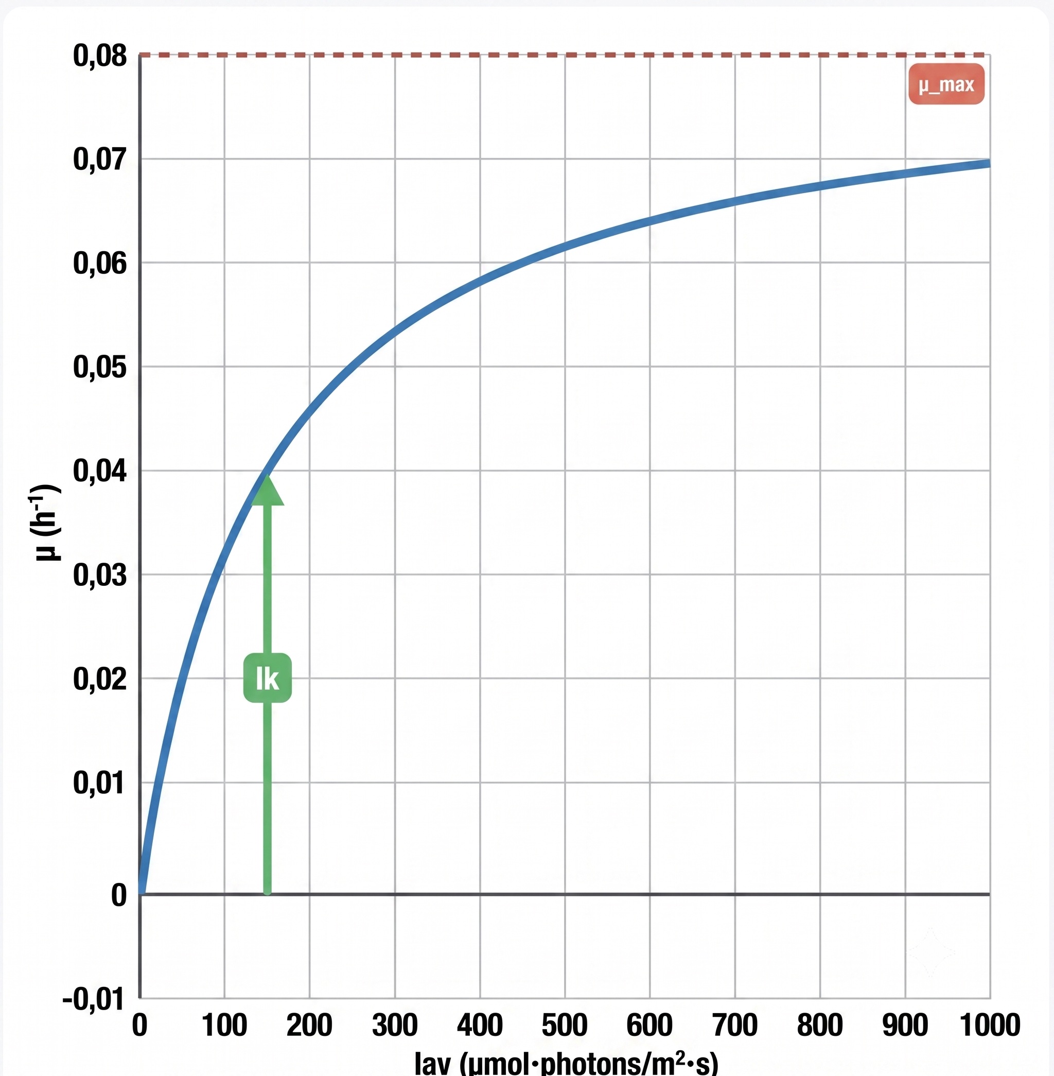Tamiya growth model (1953).

In this case, we need a light-limitation growth model of the form:

$$\begin{align} \large \mu= \frac{\mu_{max} \cdot I}{I_k+I } \tag{1.4.3} \end{align}$$

This is the Tamiya model, a light-limitation growth model for microalgae analogous to the Monod model for heterotrophic organisms.

This is a simple two-parameter model that gives the $\mu - I$ relationship when its two parameters are known:

• $\boldsymbol{\mu_{max}}$: Maximum specific growth rate. This is the $\mu$ reached by the organism when there is no limitation to growth.

• $\boldsymbol{I_k}$: Saturation constant. Controls the point at which substrate saturation occurs. With a high $I_k$, the microalga requires a high light level $I$ to become saturated.

These equations are very useful for PBR design as they allow $\mu$ to be calculated from environmental conditions. However, the Tamiya model is overly simple and does not reproduce the $\mu - I$ relationship in microalgae well. Other models have therefore emerged to compensate for Tamiya's shortcomings.

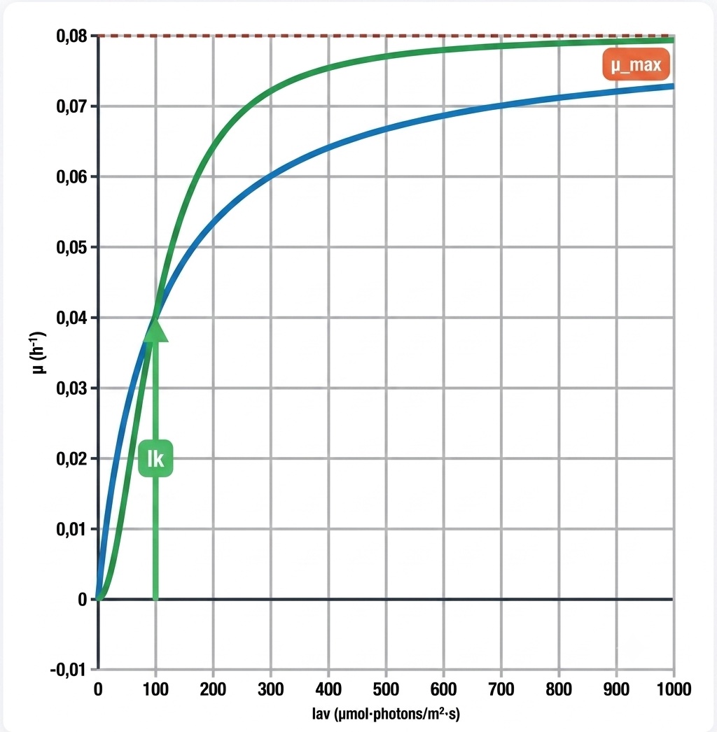Tamiya and Molina et al. growth models compared.

An alternative to Tamiya is the equation proposed by Molina et al.:

$$\begin{align} \large \mu= \frac{\mu_{max} \cdot I^n}{I_k^n+I^n } \tag{1.4.4} \end{align}$$

This is the Tamiya model modified with a shape parameter n, analogous to the Moser model for heterotrophic organisms.

The parameter n allows the Molina et al. model to display a linear $\mu - I$ zone and saturate more rapidly when n > 1.

• $\boldsymbol{n}$: Controls the shape of the $\mu - I$ curve.

The adjacent figure compares the Tamiya and Molina et al. models with n = 2. The other parameters, $\mu_{max}$ and $I_k$, are kept constant. Both models tend towards $\mu_{max}$ as $I$ increases and reach $\mu = \mu_{max}/2$ when $I = I_k$. However, the two models are clearly different.

Light-limitation growth models are essential for PBR design. They will be studied in some depth in Lesson 3.

- Light availability

As discussed in the two preceding sections, to design the PBR we need to know the relationship between $\boldsymbol{C_b}$ and $\boldsymbol{\mu}$.

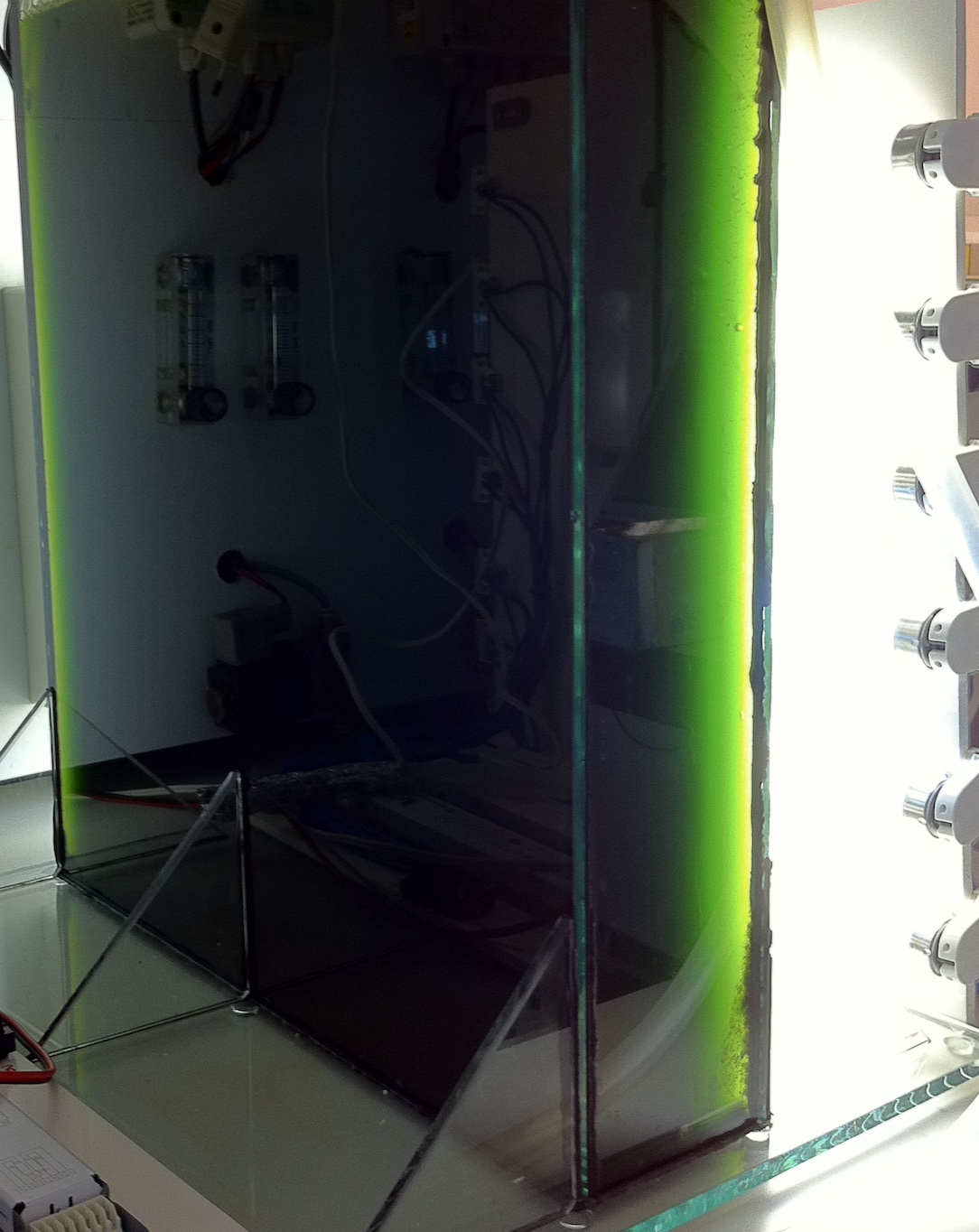Irradiance gradient in a flat-panel PBR with dense culture.

We have seen that light-limitation growth models relate $\boldsymbol{\mu}$ and $\boldsymbol{C_b}$.

It remains, therefore, to relate $\boldsymbol{C_b}$ to $I$ (light availability), which is the limiting substrate. In PBRs, this is the equivalent of the "limiting substrate balance" in conventional bioreactor design.

However, quantifying $I$ in dense cultures presents additional difficulties for the following reasons:

• Microalgae absorb light very intensely.

• In dense cultures (high $C_b$), intense irradiance gradients ($I$) develop.

• Highly illuminated zones coexist with virtually dark zones.

• Therefore, it is not straightforward to assign a value to $I$ that can be used in growth models.

As can be observed in the adjacent image, irradiance gradients are very intense and are by no means negligible.

Light availability $(I)$ depends on the incident irradiance $(I_o)$, the biomass concentration $C_b$, the type of microalgae strain and the geometry of the PBR. In the example shown in the adjacent image, it is obvious that depth (thickness) favours the presence of dark zones and vice versa.

To characterise light in a PBR, we need to quantify two elements: the irradiance profile and the average irradiance.

Irradiance profile

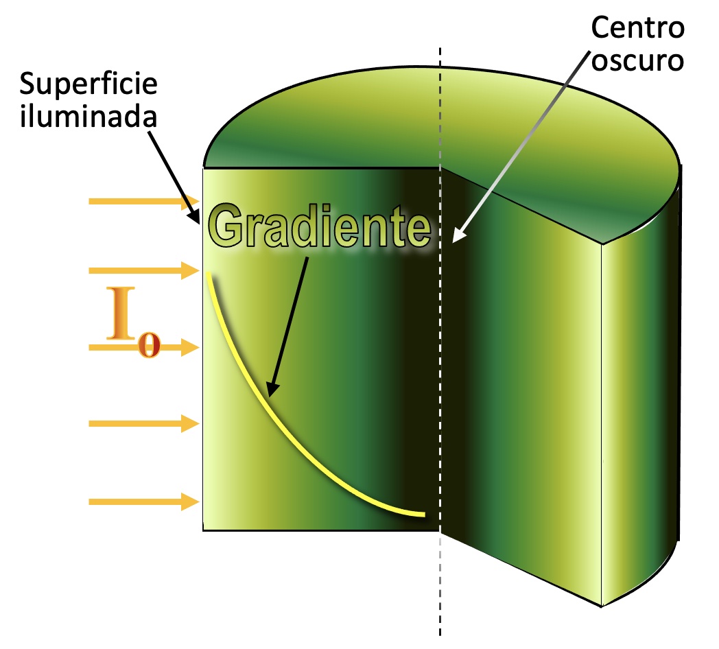Light gradient in a cylindrical PBR.

Unlike other substrates, irradiance $I$ is not homogeneously distributed throughout the (photo)bioreactor.

Especially when operating with dense cultures, there is an irradiance value at every point in the PBR. The relationship between position and irradiance is called the irradiance profile: $\boldsymbol{I(\vec{r})}$.

Obviously, this function $I(\vec{r})$ will depend on the geometry, which will differ depending on whether the system is flat or cylindrical, and will depend on how the light is incident (perpendicular, oblique, direct, diffuse, etc.).

Flat geometry with perpendicular incidence is the simplest case because $\vec{r}=x$.

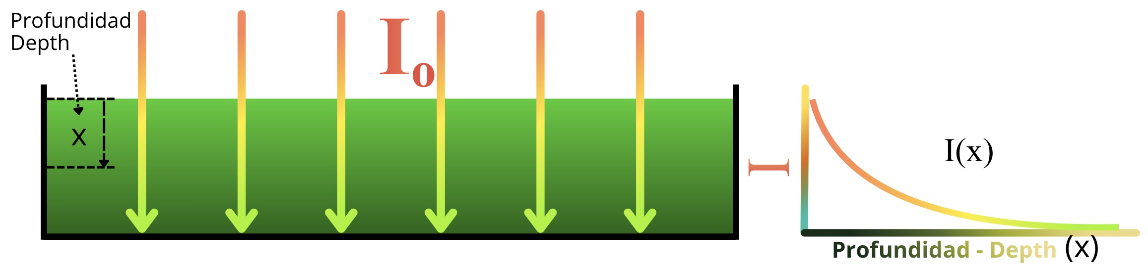
Light gradient in a flat-panel PBR with perpendicular incidence.

In this type of system, the irradiance profile can be satisfactorily represented by the Beer-Lambert law:

$$\Large I_p(x)=I_o \cdot e^{-k_a \cdot C_b \cdot x}$$

This reveals that light attenuation depends on three elements:

• the optical path length x

• The biomass concentration $\boldsymbol{C_b}$

• The extinction coefficient $\boldsymbol{k_a}$, which contains the optical properties of the microalga and which we will study in detail in Lesson 2.

Fortunately, the Beer-Lambert Law can be adapted to other geometries and situations (different from flat geometry with perpendicular light incidence). We will devote a large part of Lesson 2 to this.

Finally, it should be noted that $I(x)$ or $I_p(x)$ represents a major step forward in the description of light in a PBR, which is essential but not sufficient. To complete the description of light, we will also need to calculate an average, as described below.

Average irradiance

To be able to design PBRs, a method is needed for assigning a value to light availability from the irradiance profile $I_p(x)$.

The most obvious approach is to calculate an average: take a number of values of $I$ at various points in the PBR (for example $I_1$, $I_2$, $I_3$, $I_4$, $I_5$) and compute the average:

$$\large I_{average}=\frac{I_1+I_2+I_3+I_4+I_5}{5}$$

The situation is shown in the figure below:

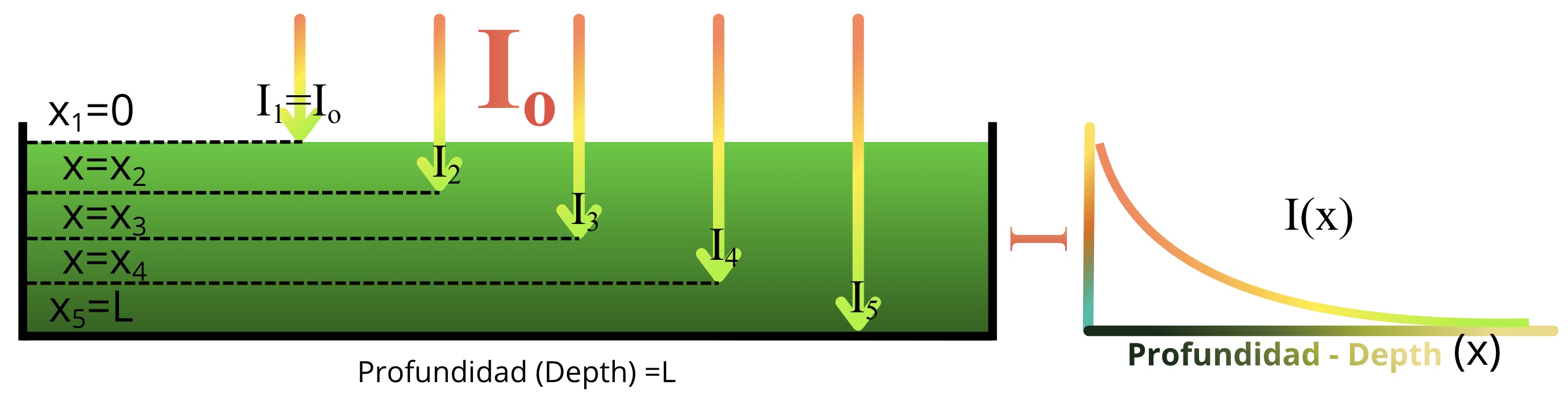
$I_p$ at five depths between the surface (x=0) and the bottom (x=L) of the PBR.

Where $I_p$ has been measured or calculated at several equally spaced levels ($x_1$, $x_2$, $x_3$, $x_4$, $x_5$) and the average has been computed. However, this procedure is inconvenient for several reasons:

• The number of points chosen is arbitrary.

• There is no guarantee that n points adequately represent $I_{average}$.

• It is difficult to standardise. For it to be a comparable value, everyone would need to take the same number of points.

This procedure can be generalised to n points with the formula:

$$\large I_{\text{average}}=\frac{\displaystyle\sum_{i=1}^{n}I_p(x_i)}{n}$$

What interests us is the value that $I_{average}$ takes as $n\to \infty$. This value is what we call average irradiance $\boldsymbol{(I_{av})}$. This is a central concept in PBR design, which we will learn to calculate in Lesson 2.

- Productivity

We already defined volumetric productivity $\boldsymbol{P_b}$ as:

$$\large P_b=\frac{dC_b}{dt}$$

And noted that it is the parameter we want to optimise in industrial PBRs, since it is the one that guarantees the greatest economic return on the investment made in a PBR, which normally depends on its installed volume $\boldsymbol{V_R}$.

From the above equation and the definition of $\mu$, it follows that:

$$\large P_b= \mu \cdot C_b$$

As already discussed in Section 1.1, you may be tempted to increase both $C_b$ and $\mu$ simultaneously. However, this is impossible. In optically dense cultures such as industrial ones:

• High $\mu$ requires high $I$ $\Rightarrow$ low $C_b$.

• High $C_b$ results in low $I$ $\Rightarrow$ low $\mu$.

There is a "conflict" between the two variables. The solution is to find the intermediate point at which $\boldsymbol{(P_b)_{max}}$ is achieved. The relationship between $C_b$, $\mu$ and $P_b$ can be seen more clearly in the graph below:

Productivity (Pb), Cb and µ as a function of I

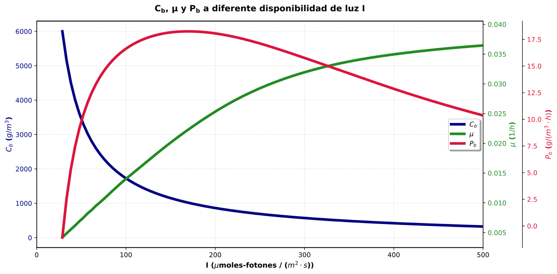
As can be seen, it is neither easy nor obvious to find the point at which $(P_b)_{max}$ occurs, so a quantitative analysis is essential. We will carry this out in Lesson 4 using the concepts learned in Lessons 2 and 3.

Finally, the overall PBR productivity $(\boldsymbol{F_b})$ (I like to use the term "Biomass Output Rate") is:

$$\large F_b= P_b \cdot V_R$$

And, obviously:

$$\large \boldsymbol{(F_b)_{max}= (P_b)_{max} \cdot V_R}$$

This is the operating point of an optimised PBR.

PBRs are designed for their optimal conditions, since otherwise we would be losing efficiency, oversizing the PBR for the required production and incurring additional capital and maintenance costs.

- Mass balances: PBR design and optimisation

PBR design requires one more element: at least one mass balance on the biomass.

The mass balance is the element that ultimately allows the variables $\mu$, $C_b$ and $I$ to be linked together. The expression of the general mass balance (GMB) is:

General mass balance

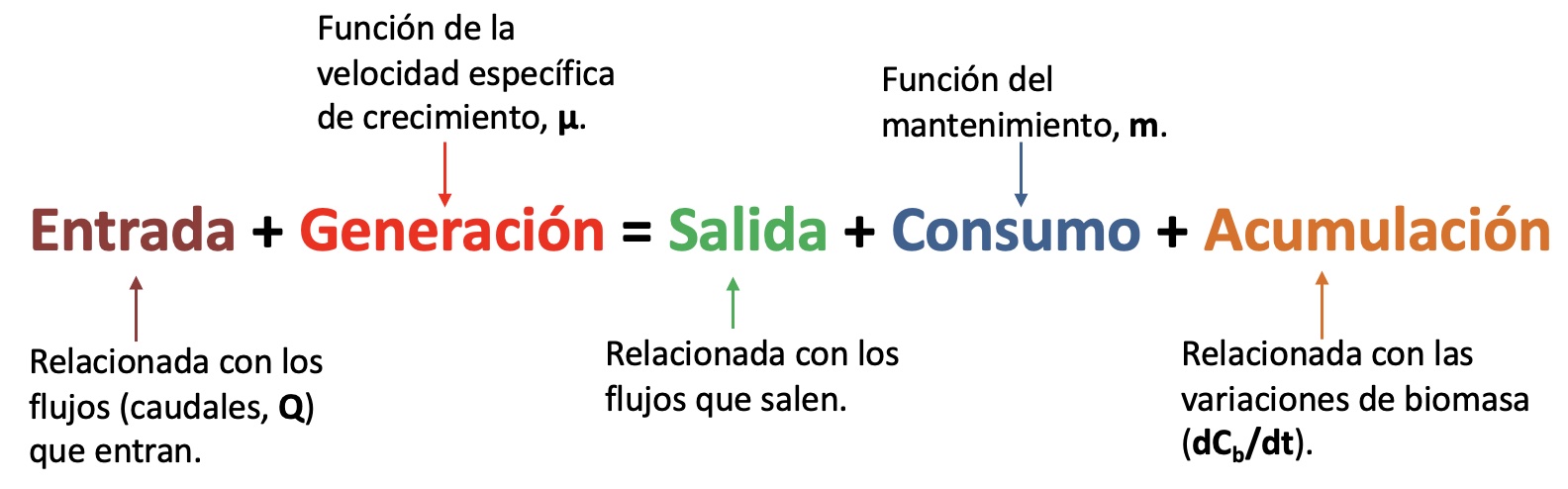
The application of the GMB depends on the photobioreactor and the cultivation mode, which can be:

• Batch or fed-batch culture.

• Continuous culture.

• Semi-continuous culture.

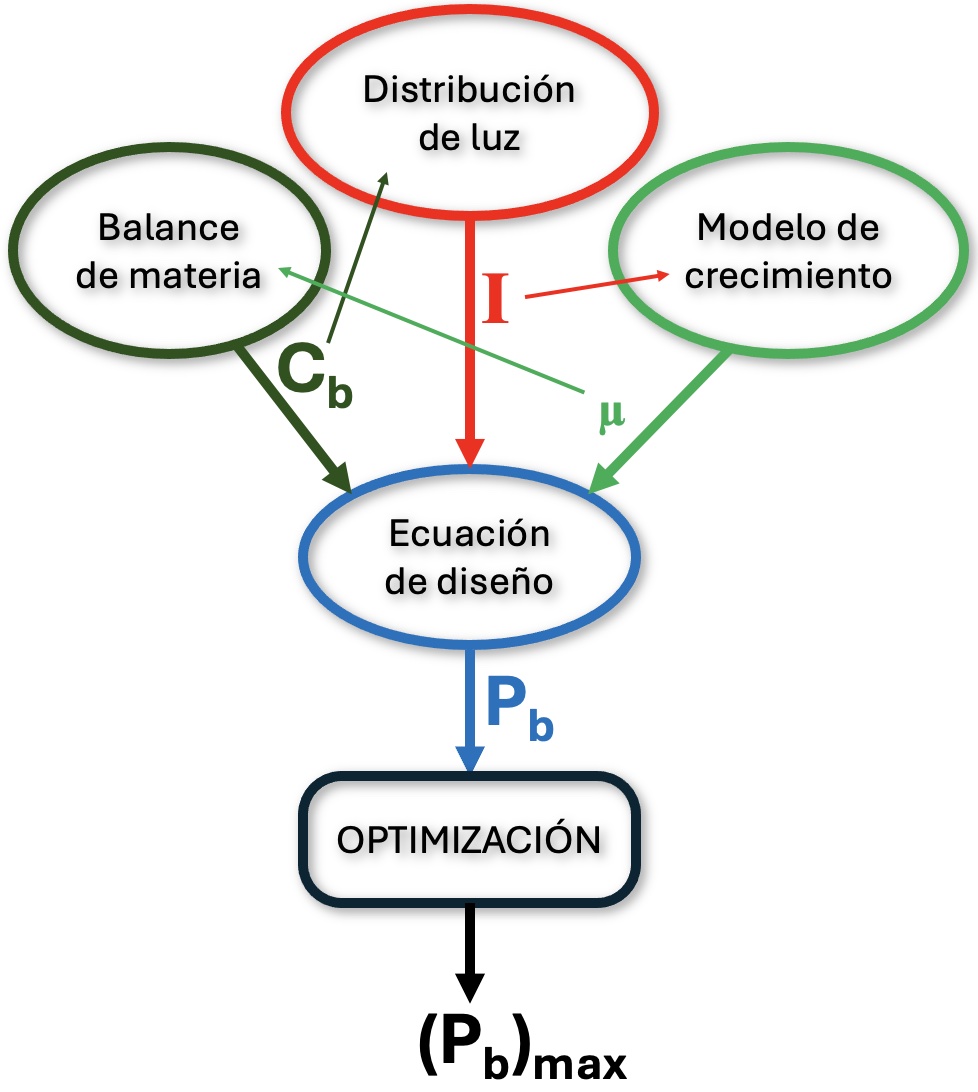Design equation.

The use of the GMB together with light-limitation growth models and light availability evaluation equations allows the design equation of the PBR to be obtained.

The design equation allows productivity $(P_b)$ to be obtained as a function of the operating conditions which, depending on the cultivation mode, may be:

• The dilution rate $\boldsymbol{D}$: $(D=Q/V_R)$, where Q is the dilution flow rate, in the case of flow-through systems (continuous culture).

• $\boldsymbol{t}$: operating time, in batch systems.

• $\boldsymbol{t_c}$: cycle time in semi-continuous systems.

PBR optimisation will be covered in Lesson 4. Once $(P_b)_{max}$ has been found, the nitrogen, $CO_2$ requirements and $O_2$ removal needs remain to be calculated.

- Nutrient supply and gas exchange in PBRs

Once the PBR has been optimised, we know its volume $V_R$ and its maximum productivity $(P_b)_{max}$. Therefore, we know its maximum or optimal production $(F_b)_{max}$ (biomass output rate):

$$\large (F_b)_{max}=(P_b)_{max} \cdot V_R$$

Which we will call $F_b$ in the following equations. Using the stoichiometric coefficients derived in Section 1.2:

• Oxygen: $\large \Psi_{O_2/biomass}$

• Carbon $(CO_2)$: $\large \Psi_{CO_2/b}$

• Nitrogen: $\large \Psi_{N/b}$, which can be converted to nitrate, ammonium or any salt of these ions serving as a N source.

With these coefficients, it is straightforward to estimate $N$ and $CO_2$ consumption:

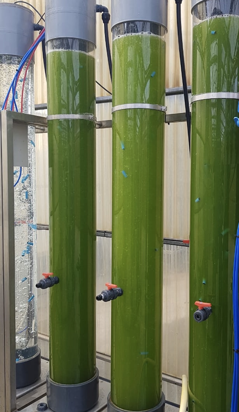Bubble-sparged columns.

• $\boldsymbol{F_N}=V_R \cdot P_b \cdot \Psi_{N/b}$

• $\boldsymbol{F_{CO_2}}=V_R \cdot P_b \cdot \Psi_{CO_2/b}$

And $O_2$ generation:

• $\boldsymbol{F_{O_2}}=V_R \cdot P_b \cdot \Psi_{CO_2/b}$

Nitrogen is a salt supplied in dissolved form, either as part of the culture medium $((F_{N})_{in}=Q \cdot (C_{N})_{in})$ in continuous cultures, or as an initial concentration of $N$ in batch cultures, a concentration that is consumed as biomass concentration increases.

On the other hand, $CO_2$ and $O_2$ must always be supplied or removed continuously, even if the culture is batch or semi-continuous.

In addition, the difficulty arises that $CO_2$ and $O_2$ are GASEOUS nutrients and (by-)products, which makes it necessary to carefully design gas transfer in PBRs, as we will see in Lesson 5.

For the design of gas transfer, the volume of the contact device (usually called the degasser, hence $\boldsymbol{V_D}$) must be determined, and for this the overall mass transfer coefficient $(\boldsymbol{K_La})$ must be known.

For correct gas transfer, $V_D$ must be found such that both conditions are satisfied:

• $\boldsymbol{O_2}$ transfer: ${F_{O_2}}=V_D \cdot (K_La)_{O_2} \cdot (C_{O_2}-C^*_{O_2})$

• $\boldsymbol{CO_2}$ transfer: ${F_{CO_2}}=V_D \cdot (K_La)_{CO_2} \cdot (C^*_{CO_2}-C_{CO_2})$

This completes the PBR design for biomass production, and is what will occupy us throughout Lessons 1 to 5.

Summary 1.4 - Key concepts in PBR design

Objective

Design industrial microalgae cultures in PBRs to maximise biomass, minimise resources, maintain stability and maximise products of interest.

Key concepts

1. Specific growth rate (μ)

• Defines biomass production capacity: $\mu = \frac{1}{C_b} \cdot \frac{dC_b}{dt}$
• In industrial PBRs, μ depends strongly on light (I)
• Models: Tamiya (simple) and Molina et al. (with shape parameter n)

2. Light availability

• Irradiance profile I(x): Beer-Lambert Law $I_p(x)=I_o \cdot e^{-k_a \cdot C_b \cdot x}$
• Average irradiance ($I_{av}$): mean value as n→∞
• Intense gradients in dense cultures

3. Productivity ($\boldsymbol{P_b}$)

• $P_b = \mu \cdot C_b$
• Conflict: high μ requires high I → low $C_b$, and vice versa
• Objective: find $(P_b)_{max}$
• Overall production: $F_b = P_b \cdot V_R$

4. Mass balance

• Links variables μ, $C_b$ and I
• Application depends on mode: batch, continuous, semi-continuous
• Yields the PBR design equation

5. Nutrient and gas supply

• Once optimised: $F_b = P_b \cdot V_R$
• Consumption: $F_N$ and $F_{CO_2}$ using stoichiometric coefficients
• Generation: $F_{O_2}$
• Gas transfer: design of $V_D$ using $K_La$

- Questions and problems.