 |  |
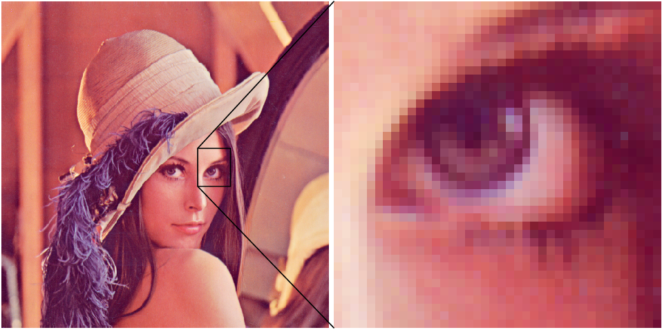
| Homer.ppm (1,467,663 bytes) | Homer.j2c (12,101 bytes (122 times smaller)) |
| | |
| Homer.ppm (1,467,663 bytes) | Homer.j2c (12,101 bytes (122 times smaller)) |
| (1) |
which when the dinamic range of the RGB components is can be approximated by
| (2) |
in order to avoid the floating point computations.

| R, bpp | G, bpp | B, bpp |
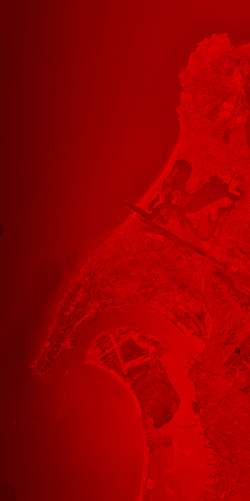 | 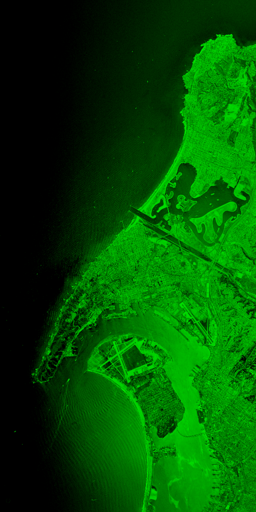 | 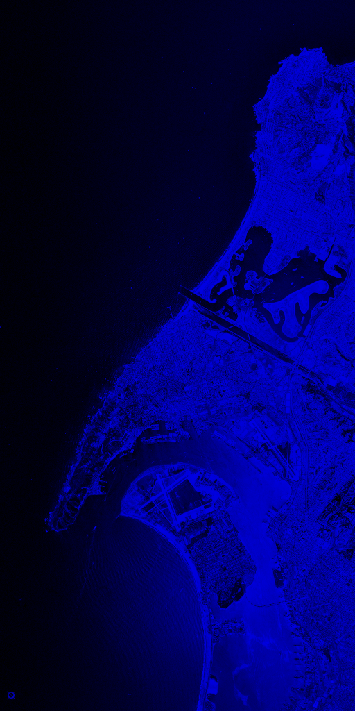 |
| Total 21,37 bpp | ||
| Y’, bpp | Cb, bpp | Cr, bpp |
 |  |  |
| Total 18,79 bpp | ||
| (3) |
where is the number of bits/pixel and MSE (Mean Squared Error) is
| (4) |
where is the number of pixels, s[] is the -th () point of the image and is the -h point of the reconstructed image.
| | 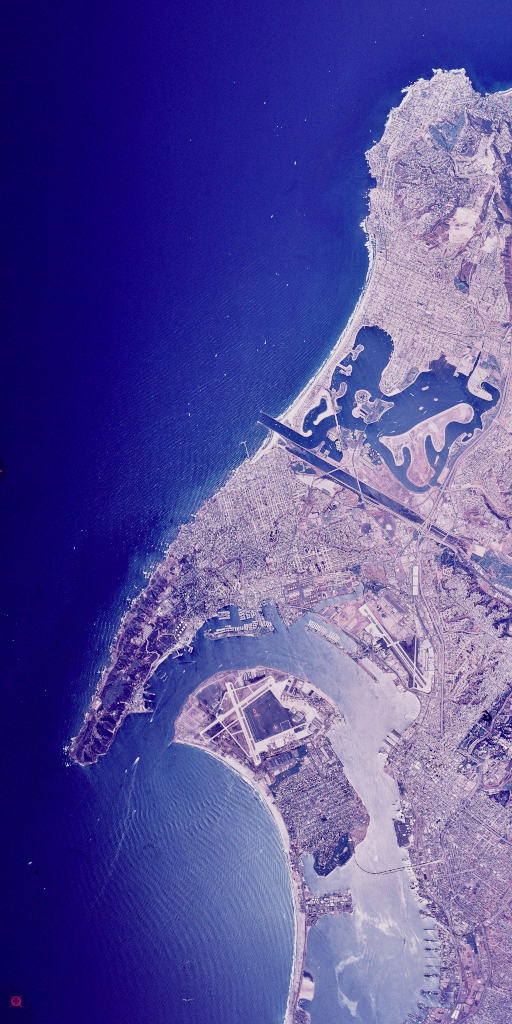 |
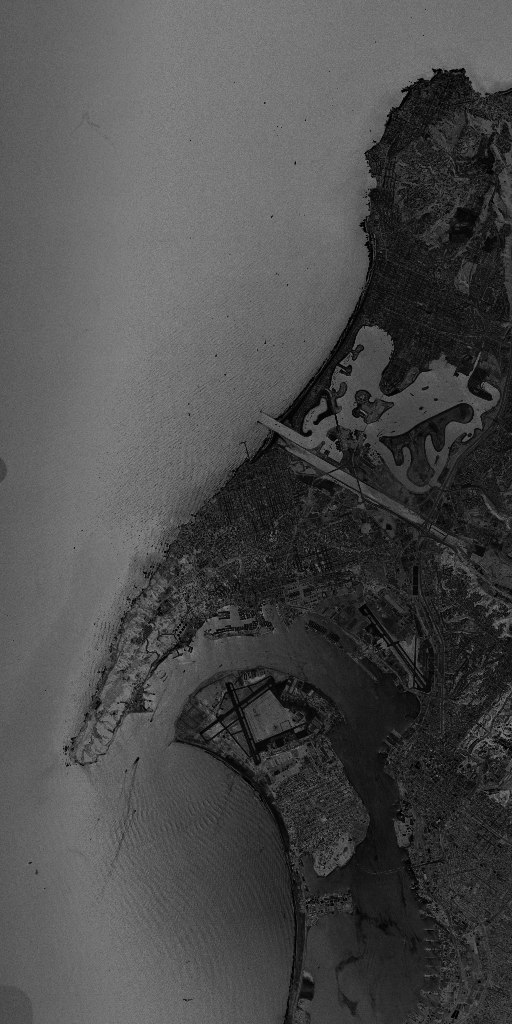
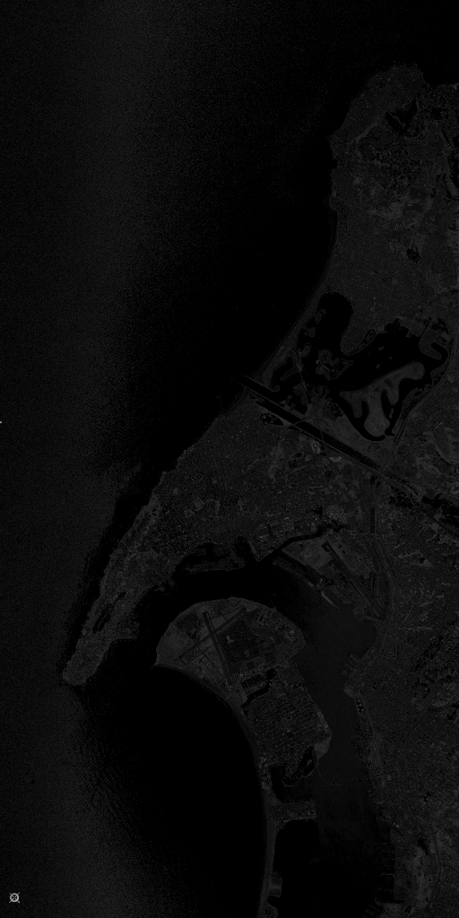
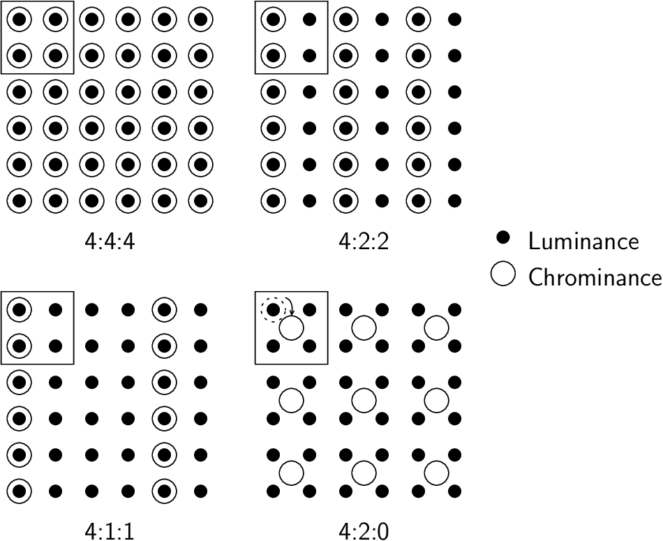
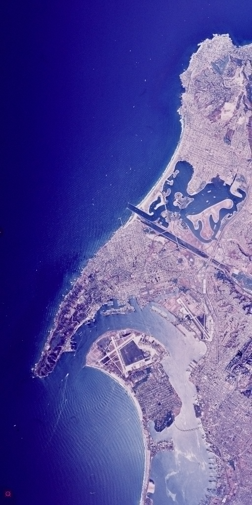
| Original (4:4:4) | Subsampled (4:2:0), PSNR dB |
| | 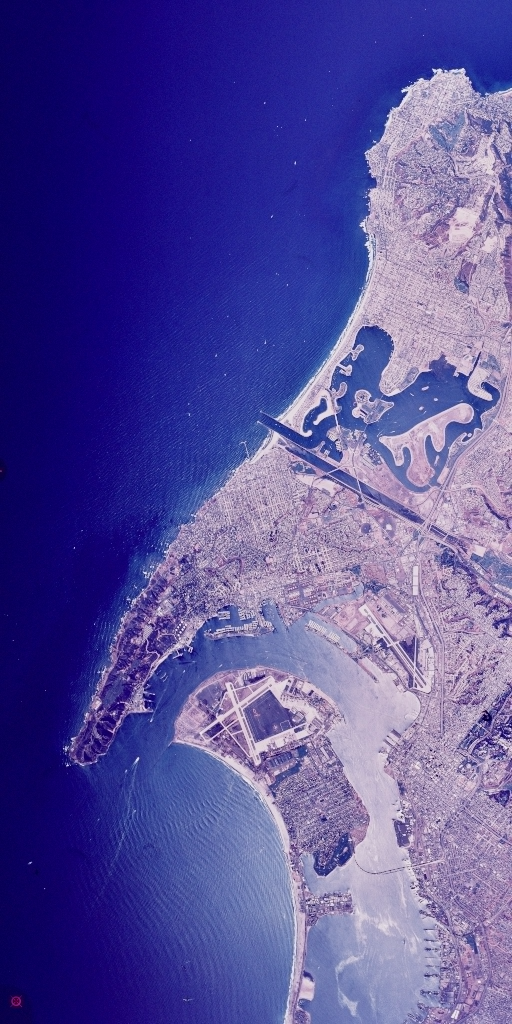 |
| Original (8:8:8) | Subsampled (8:2:0), PSNR dB |
| |  |
| Original (16:16:16) | Subsampled (16:2:0) PSNR dB |
| (5) |
and the inverse transform is
| (6) |
where is the number of pixels, and denotes the -th pixel of the image , and
- - - 
- - - 
- - - 
- - - 
- - - 
Where
| (7) |
and
| (8) |
| (9) |
and
| (10) |
where if the -th sample of .
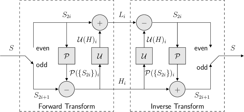
| (PredictionStep) |
| (UpdateStep) |
and
where represents the one sample delay function.
| (11) |
where represents the Euclidian Norm (also known as the L Norm) of the sample , that in a general case could be a complex number.
| (12) |
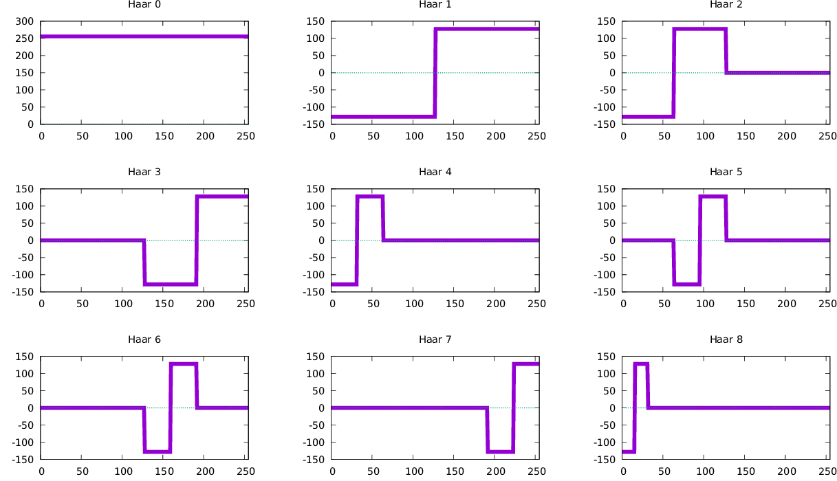
| (HaarL) |
and the -th sample of the high-frequency subband as
| (HaarH) |
If Lifting is used,
| (HaarLLifted) |

- - - 
- - - 
- - - 
- - - 
- - - 
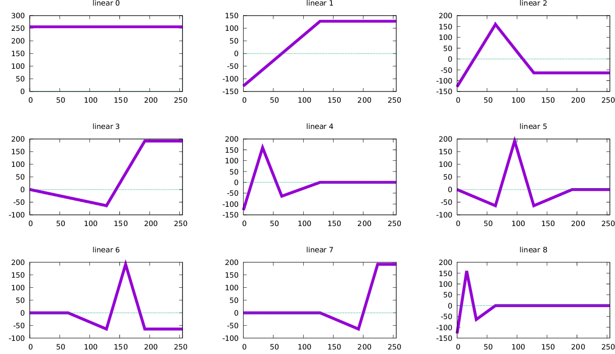
| (5/3L) |
and the -th sample of the high-frequency signal is computed by
| (5/3H) |
that, if we use Lifting, it can be also computed using less operations by
| (5/3LLifted) |

- - - 
- - - 
- - - 
- - - 
- - - 
| (13/7H) |
and (the lifted) calulus of the -th sample of the low-frequency signal is
| (13) |

- - - 
- - - 
- - - 
- - - 
- - - 
![]()
[1] M. D. Adams and F. Kossentini. Reversible Integer-to-Integer Wavelet Transforms for Image Compression: Performance Evaluation and Analysis. IEEE Trans. Image Process., 9(6):1010–1024, 2000.
[2] M.D. Adams. Reversible Wavelet Transform and their Application to Embedded Image Compression. PhD thesis, A,A,Sc, University of Waterloo, 1993.
[3] A. Haar. Zur Theorie der orthogolanen Funktionen-Systeme. Mathematische Annalen, 69:331–371, 1910.
[4] The Joint Photographic Experts Group (JPEG). Recommendation T.81: Digital Compression and Coding of Continuous-tone Still Images. International Telecommunication Union (ITU), September 1992.
[5] A.M. Marcos. Compresión de imágenes. Norma JPEG. Editorial Ciencia 3, 1999.
[6] Majid Rabban, Rajan L. Joshi, and Paul W. Jones. The JPEG 2000 Suite, chapter JPEG 2000 Core Coding System (Part 1). WILEY, 2009.
[7] Ana Sovic and Damir Sersic. Signal decomposition methods for reducind drawbacks of the dwt. Engineering Review, 32(2):70–77, 2012.
[8] W. Sweldens and P. Schröder. Building Your Own Wavelets at Home.